Outline
1. Definition of Hydrological Science
2. Why Study Surface Hydrology?
3. Hydrological Cycle
1. What is hydrological science?
From COHS, 1991.
A Distinct Geoscience
Over the past 60 years, the evolution of hydrologic science has been in the direction of ever-increasing space and time scales, from small catchment to large river basin to earth system, and from storm event to seasonal cycle to climatic trend. Hydrologic science should be viewed as a geoscience interactive on a wide range of space and time scales with the ocean, atmospheric, and solid earth sciences as well as with plant and animal sciences. To establish and retain the individuality of hydrologic science as a distinct geoscience, its domain is defined as follows:
Continental water processes-- the physical and chemical processes characterizing or driven by the cycling of continental water (solid, liquid and vapor) at all scales (from the micropores of soil water to the global processes of hydroclimatology) as well as those biological processes that interact significantly with the water cycle.
(This restrictive treatment of biological processes is meant to include those that are an active part of the water cycle, such as vegetal transpiration and many human activities, but to exclude those that merely respond to water, such as the life cycle of aquatic organisms.)
Global Water Balance-- the spatial and temporal characteristics of the water balance (solid, liquid and vapor) in all compartments of the global system: atmosphere, oceans and continents.
(This includes water masses, residence times, interfacial fluxes, and pathways between compartments. It does not include those physical, chemical or biological processes internal to the atmospheric and ocean compartments.)
The scope of this class (i.e. surface water hydrology) deals with those continental hydrological processes occurring at or near the land surface
Hydrologic science deals with the waters of the earth, including their
- occurrence
- distribution
- circulation
- chemical and physical properties
- reaction with their environment
- relation to living things
The science of hydrology embraces the full life history of water on the earth.
Hydrology is closely related to other natural sciences:
- Precipitation and evaporation require knowledge of climatology and meteorology
- Infiltration and evaporation require knowledge of soil science
- Transpiration requires knowledge of biological process
- Groundwater flow requires insights into geology
- Surface runoff requires knowledge of geomorphology
- Streamflow requires knowledge of fluid mechanics
It is a multi-disciplinary science since water interacts (i.e. it is important to and affected by)
- physical processes
- chemical processes
- biological processes
within all compartments of the earth system, i.e. the
- atmosphere
- oceans
- solid earth
- ice sheets
- rivers
- lakes
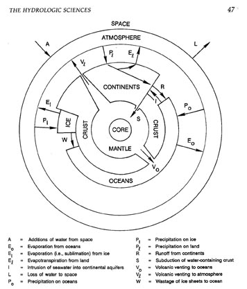
as shown in COHS (1991) Figure 2.4.
2. Why do we need to study surface hydrology?
Since water pervades the earth system and interacts with its various components on a range of spatial and temporal scales, land surface hydrology plays a critical, if not central role, in the interactive functioning of the earth system. Therefore, it is tightly coupled to numerous earth system processes ( e.g. climate, weather, biogeochemistry, ecosystem dynamics).
For example, at large (e.g. continental) scales, soil water stored in soils near the land surface exerts a major control on climatic and weather processes by affecting land surface temperatures and by supplying moisture to the atmosphere via evapotranspiration. We are now suspecting that runoff from the continents affects ocean circulation, which via their control of sea surface temperatures, that have a major impact on climate.
At regional scales, land use practices such as irrigation, grazing, and deforestation have feedbacks to regional hydrology, climate, and weather.
At smaller scales, practical issues of water resources management, flood control
flood forecasting, water supply forecasting and groundwater quality require an intimate knowledge of surface hydrologic processes to really grasp the big picture and to function effectively in water resources careers in engineering/consulting/planning, government or academia.
Given the above background, a primary goal of this class is to educate you with the perspective that the hydrologic cycle is a fundamental earth system cycle, interactive with other earth system components across a broad range of spatial-temporal scales. We’ll see that this cross-disciplinary theme will be echoed throughout the semester.
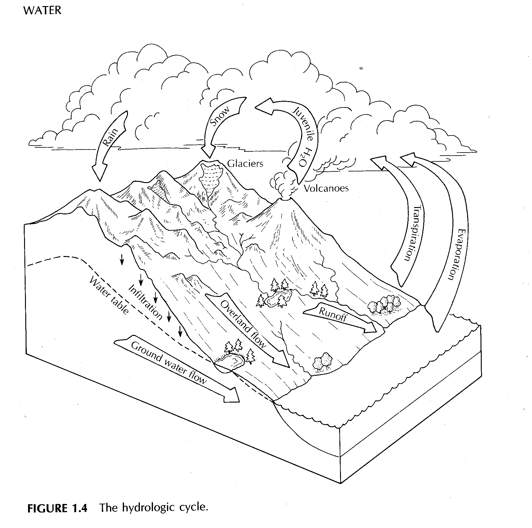
The pathway of water as it moves in its various phases, through the atmosphere, over and through the land, to the ocean, and back to the atmosphere, is known as the hydrological cycle. It is the most fundamental principle of hydrologic science. These pathways are shown graphically in Figure 1.4 of Fetter, 1994.
Precipitation falling on land takes various pathways through the hydrological cycle
Some of the rain will drain across the landscape toward stream channels as overland flow (runoff).
Some of the rain will seep into porous soils through infiltration.
Below the land surface, the region where soil pores contain both air and water is called the unsaturated zone (zone of aeration, vadose zone).
Water stored in the unsaturated zone is called soil moisture (soil water). A measure of the amount of water in the soil is called the moisture content, or soil water content.
Near surface soil moisture is extracted by roots, and is then transpired. Water in the unsaturated zone can also migrate back to the land surface to evaporate.
Under some conditions, water can flow laterally in the unsaturated zone, e.g. through macropores, a process known as interflow.
Some water in the unsaturated zone is pulled downward by gravity drainage (percolation).
At some depth, the pores of the soil are saturated with water. The top of the saturated zone is called the water table
Water stored in the saturated zone is called groundwater. It moves through the soil layer as saturated subsurface flow (baseflow, groundwater flow) until it discharges as a spring, seeps into a pond or stream, or the ocean.
Water flowing in a stream derives from overland flow, from groundwater that has seeped into the stream channel, and perhaps from interflow.
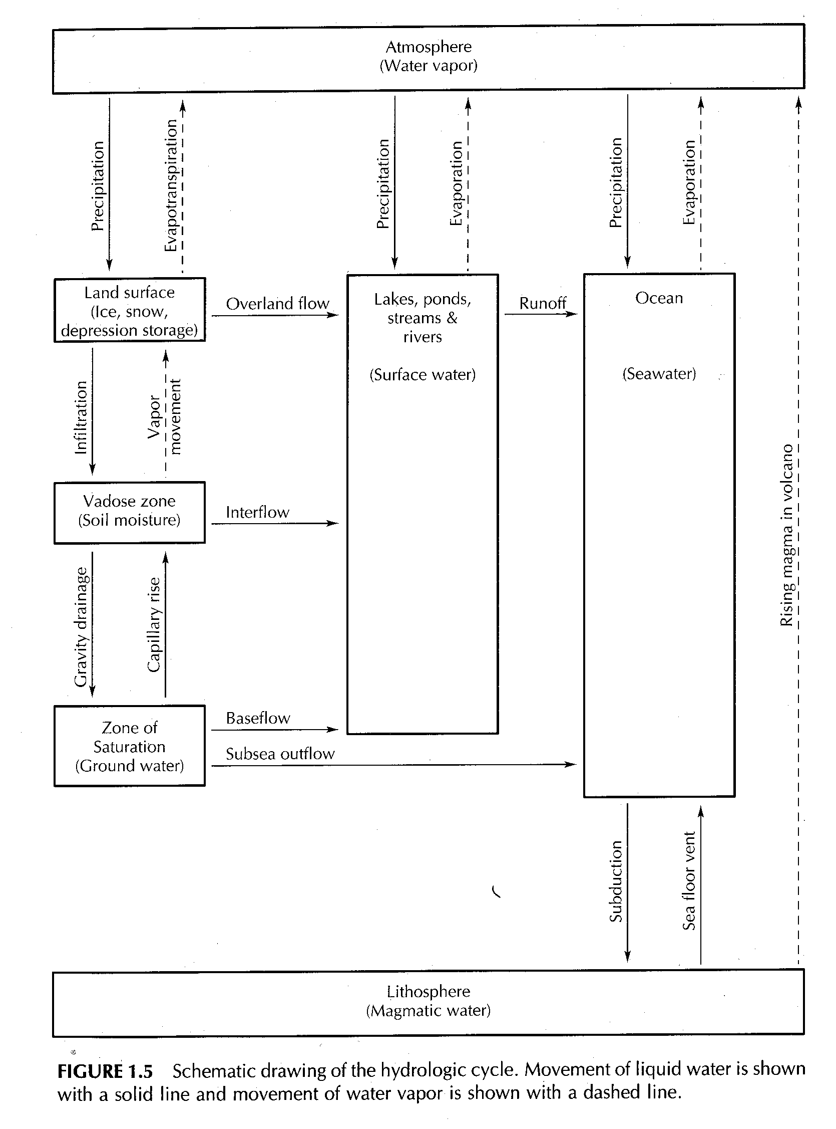
Many of the pathways that water takes once on land have specific direction. For example, baseflow, overland flow, streamflow are topographically-driven downslope. Others are more ubiquitous, provided there is a moisture source (e.g. infiltration occurs over large spatial areas after rain events; evaporation occurs from soil, plants, from water intercepted by plant canopies, and from any open water bodies (oceans, lakes, streams)). See Fetter, (1994) Figure 1.5.
References
Committee on Opportunities in the Hydrologic Sciences (COHS), Water Science and Technology Board, Commission on Geosciences, Environment and Resources, National Research Council, 1991. Opportunities in the Hydrologic Sciences, , National Academy Press, Washington, DC.
Fetter, C. W., 1994. Applied Hydrogeology, Macmillan College Publishing Co., New York.
Back to top of page
2: Hydrology Basics I
Outline
1. Conservation Equations
2. Water Balance Examples
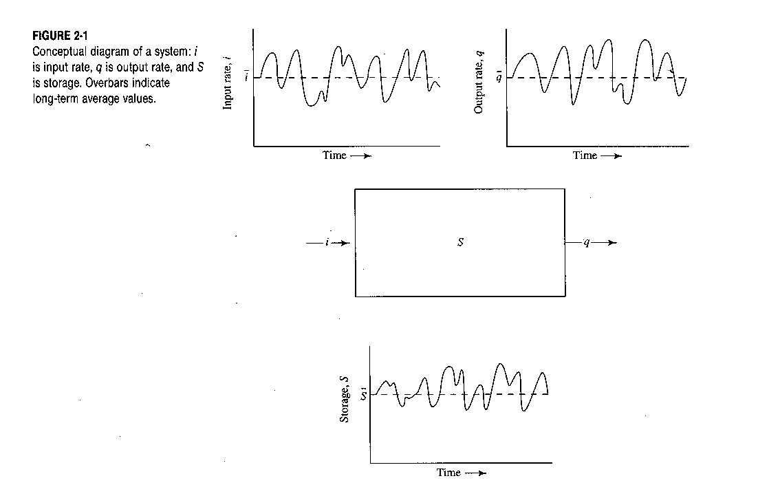
A system is any conceptually-defined region of space capable of
A system is sometimes called a control volume. See Dingman, 1994, Figure 2-1 for a conceptual diagram of a system.
A conservative quantity is one that cannot be created or destroyed within the system, for example
The basic conservation equation states:
The amount of a conservative quantity entering a control volume during a defined time period, minus the amount leaving the volume during the time period, equals the change in the amount of the quantity
This basic conservation equation is in fact a generalization of the conservation of mass, Newton's first law (conservation of momentum) and the first law of thermodynamics (conservation of energy)
Stated more simply
remembering of course that this is only true for
Other useful forms can be obtained by dividing by DT as shown in the text, yielding
dS/dt = i - q
where i and q are the instantaneous rates of inflow and outflow and dS/dt is the instantaneous rate of change of storage.
Note now that there are no restrictions on the size of the control volume or the length of the time period so that the conservation equations are scale and time independent
When applied to problems of the mass of water moving through the hydrological cycle, they are called water balance equations. Since the conservation equations are space-time independent, we can apply them from the point, or infinitesimally small spatial scales, up to the global scale, and on anything from instantaneous to very long time scales. When the conservation equations are applied to energy they are called the energy balance equations.
Since the conservation equation is scale independent, we could apply it at
Examples from class: the root zone of a soil column, a water balance on a lake, and a watershed on a drainage basin.
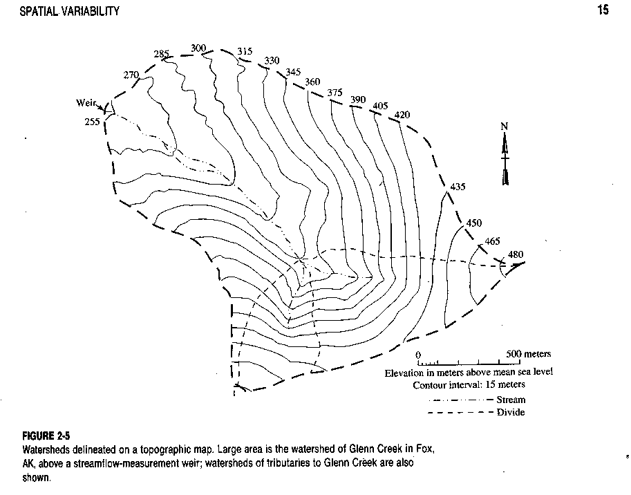
With respect to the drainage basin example, we first need to define a drainage basin (watershed, catchment, river basin) as the area which drains through a particular point in a stream network, i.e. it is the area that topographically appears to contribute all the water that passes through a given cross section of stream. Drainage basins are outlined by topographic divides. These are the boundaries which delimit watersheds. See Dingman, 1994, Figure 2-5 for an example of a watershed delineated on a topographic map.
Watersheds can be delineated for any point on the stream network, so there are an infinite number of watersheds that can be drawn for any stream. Delineation is most often done manually, but can now be done automatically using digital elevation models (DEMs). DEMs are simply computer data files that give land-surface elevations at grid points.
Regional water balance example
The regional water balance is the application of the water balance equation (conservation equation) to a watershed (or to any land area such as a state or continent).
The watershed area delimited by its divide is the upper surface of the control volume; the sides of the volume extend vertically downward from the divide some indefinite distance assumed to be below the level of significant ground-water movement. (See Dingman, 1994, Figure 2-6)
From Dingman (1994) Figure 2-6 we can write the water balance equation for watershed
DS = I - Q
Inputs Outputs
Precipitation(P) Streamflow(Q)
Groundwaterout(GWo)
DS = P + GWi - (Q + ET + GWo)
Choice of Dt. Choose Dt for your problem of interest -- instantanoeous, daily, monthly, seasonal, annual, etc. Since many of these variables are hard to quantify over large areas (e.g. ET, GWi,o), one trick is to eliminate some of the unknowns. For example, if Dt is taken over a long enough period of time (e.g. annual) then DS can be taken as zero.
Estimation of regional ET. One of the most common applications of the regional water balance approach is in estimating regional ET. Additional assumptions are required to simplify the draingage basin water balance equation: assume that surface water divides are equal to groundwater divides, and take GWi as zero. Then we can rewrite water balance as
P - Q - ET - GWo= 0
Assume GWo is negligible (since much of the groundwater leaving the basin may in reality leave as baseflow). Then
P - Q - ET = 0
(A note on units: Water balance variables such as P, or ET are frequently given as depths (L), i.e. volumes (L3) divided by the area (L2) over which they fell. This depth quantity could be further divided by the duration of Dt to get units of L/T)
Sources of error in the regional estimation of ET: model and measurement error introduce uncertainty into the water balance which propagates into, e.g. estimated ET.
Model error: the omission of terms in the basic water balance equation:
- e.g. GWout: Could be a potentially significant term. It is less important as watershed size increases since smaller watersheds tend to drain into larger ones.
- e.g. DS=0: try to choose long periods or two times when storages are likely to be equal, e.g. after a very long rain that saturates the soil
Measurement error: uncertainties due to measurement error are always present in hydrology. Briefly, with respect to regional ET estimation, errors in P and Q will propagate into errors in ET
Precipitation: sources of error at the regional scale include measurement error at individual gaging stations, and the error due to the averaging procedure.
Streamflow: human or mechanical error associated with the particular type of stream gage.
Back to top of page
3: Hydrology Basics II
Outline
1. Energy Balance
1. Energy Balance
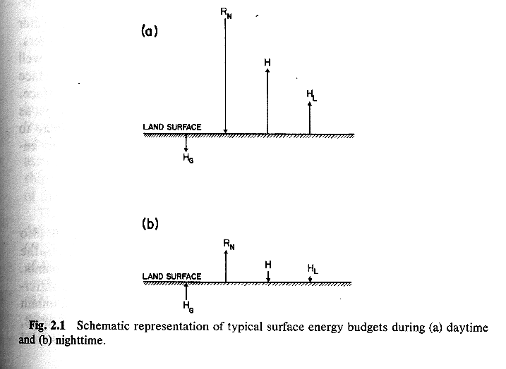
The conservation equation as applied to energy, or conservation of energy, is known as the energy balance. In general, just as we looked at how precipitation is partitioned into infiltration, runoff, evapotranspriation, etc., we can look at how incoming radiation from the sun and from the atmosphere is partitioned into different energy fluxes (where the term flux denotes a rate of tranfer (e.g. of mass, energy or momentum) per unit area).
We’ll see later (as we move through the course) that the water and energy balance are intimately linked:
Just as changes in water balance were reflected in changes in storage in water amounts (soil moisture in a root zone; level of a lake) changes in energy balance are reflected in temperature changes. Just as we wrote water balances for a number of different control volumes in the last class, we could write energy balances for the same control volumes. However, we won’t really do that because it’s beyond the scope of what we’re trying to do in this class.
Instead, we’ll look at a simplified energy budget for an ideal surface, where we define ideal as
Later, in the chapter on snow, we’ll look at the energy balance in a little more detail and add heat capacity and storage of heat in a snow layer.
The simplified energy budget for such an ideal surface is given by
Rn = H + LE + G
where
See Arya, Figure 2.1 for a schematic representation of the simplified energy budget.
Net Radiation.
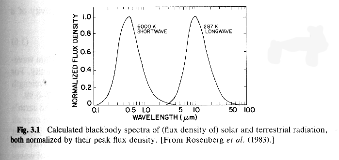
Net radiation is really composed of shortwave radiation, K, from the sun, and longwave radiation, L from the atmosphere and from the ground, so that
Rn = K + L
The radiation from the sun (solar radiation) is often referred to as shortwave radiation, and the radiation from the atmosphere and the ground (i.e. atmospheric and terrestrial radiation) as longwave radiation, since the wavelength of the electromagnetic emitted by these bodies is inversely proportional to their temperatures (See Figure 3.1 from Arya (1988)).
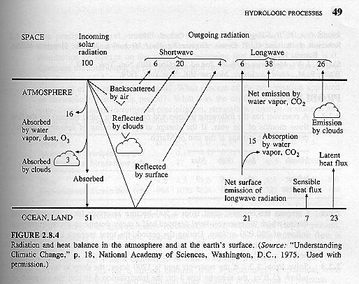
Shortwave radiation input. First, consider what happens to incoming solar radiation as it enters the earths atmosphere on the way to the surface. Figure 2.8.4 from Chow et al. (1988) shows that it may be:
The net flux of solar energy entering the land surface is therefore given as
K = Kin - Kout = Kin (1-a)
where
- K in is the incident solar energy on the surface, and it includes direct solar radiation (i.e. that which makes it through the atmosphere unscathed) and diffuse (due to scattering by aerosols and gases);
- Kout is the reflected flux;
- a is the albedo
Solar radiation is measured in specialized meteorological stations with radiometers.
However, these require careful calibration and maintenance, and consequently they are not usually available at standard weather stations. Dingman (1994), Figure E1, shows the weather stations across the US at which solar radiation data are routinely collected. A more common practice is to estimate K by modifying the clear-sky solar for the geographic location and time of year by functions of slope orientation, fraction of clouds, and fraction of vegetation (See Dingman (1994), Appendix E).
Longwave radiation input. All matter at a temperature above absolute zero radiates energy in the form of electromagnetic radiation which travels at the speed of light.
The rate at which this energy is emitted is given by the Stefan-Boltzman law
Qr = esT4
where
- Qr is the rate of energy emission per unit surface area per unit time
- T is the absolute temperature of the surface
- s is a universal constant called the Stefan-Boltzman constant
- e is a dimensionless quantity called the emissivity
The emissivity ranges from 0 to 1, depending on the material and surface texture. A surface with e equal to 1 is called a blackbody. Most earth materials have emissivities near 1.
Long-wave radiation is emitted by bodies at near earth surface temperatures (the land surface and the lower atmosphere). The net input of longwave radiation, L, is the difference between the incident flux, Lin, which is emitted by the atmosphere, clouds
and overlying vegetation canopy, and the outgoing radiation emitted from the land surface:
L = Lin - Lout
Longwave radiation is measured using radiometers. As in the case of shortwave, the instruments are rare except at intense research sites. So, it is usually estimated from more readily available meteorological information. These estimates are based on the following physics.
The flux or radiation emitted by the atmosphere is
Lin = eatsTat4
and at denotes atmosphere . Outgoing radiation is the sum of the radiation emitted by the surface and that fraction of the incoming longwave that is reflected
Lout = essTs4+(1-es)Lin
The subscript s denotes land surface. For the case of gray bodies (e<1) reflectivity equals 1 - emissivity.
Sensible Heat
H = cara/rah (Ta-Ts)
Note that this equation is essentially a conductivity times a gradient, corrected for the properties of the fluid.
- ca is the heat capacity of air
- ra is the density of air
- rah is the aerodynamic resistance to heat transport and is given by
rah = 1 / k2 u (z(m)) {ln{zm/zo}}2
- k is von Karmann's constant (0.4)
- u (z(m)) is wind speed at measurement height zm
- zo is known as the roughness height of the surface and depends of the irregularity of the surface
Latent Heat
LE = cara/ grav (es-ea)
where
- L is the latent heat of vaporization
- E is the rate of evaporation
- rav = rah
- g is the psychrometric constant, and is a function of atmospheric pressure, density of air, etc.
- es,ea are the vapor pressures measured at the surface and in the lower atmosphere
Ground Heat Flux
G = kG dT/dz
where
- kG is the thermal conductivity of the soil
- dT/dz is the vertical temperature gradient
Thermal conductivities of soils depend on soil texture, soil density, and moisture content, and vary widely in space. Owing to this variability, and the fact that dT/dz is tough to measure, G is often neglected or estimated in energy balance computations.
References
Back to top of page
4: Water in the Atmosphere
Outline
1. Composition of the Atmosphere
2. Atmospheric Circulation
3. Quantification of amount of water in atmosphere
1. Composition of the atmosphere
The atmosphere is a mixture of gases in which liquid and solid particles are suspended.
Table D-3 (Dingman, 1994) lists these various components. The major constituents, and many of the minor ones, are effectively constant in time. The variable constituents include those that are most significant hydrologically (e.g. liquid water, ice, water vapor, dusts, and CO2 ) since they effect the water and energy balance of the atmosphere and thus the formation of clouds and precipiation. The amount of water vapor in the atmosphere amounts to less than 1 part in 100,000 (0.001 %) of all the waters of the earth (0.04% of the fresh water), yet it plays a vital role in the hydrological cycle and the earth's climate system. Most of the water vapor in the atmosphere is concentrated in the lower 2 km of the atmosphere
The earth constantly receives heat from the sun as solar radiation, and emits heat back into space by back radiation. This heating of the earth is uneven, since, as seen in Dingman (1994) Figure 3-4, incoming radiation near the equator is almost perpendicular to the land surface (averaging 270 W/m2), while near the poles it strikes at a more oblique angle(averaging 90 W/m2).
Since the back radiation is proportional to the temperature of the earth's surface, which doesn't vary that much from the equator to the poles, the emitted radiation is more uniform than the incoming solar, so that in response to the imbalance, the atmosphere functions as a vast heat engine, transferring energy from the equator to the poles.
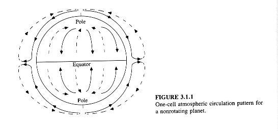
If the earth were a non-rotating sphere, the atmospheric circulation would appear as in Chow, Maidment, and Mays, 1988, Figure 3.1.1. Air would rise near the equator, travel towards the poles in the upper atmosphere, cool, and decend into the lower atmosphere. This one-cell circulation is called the Hadley circulation.
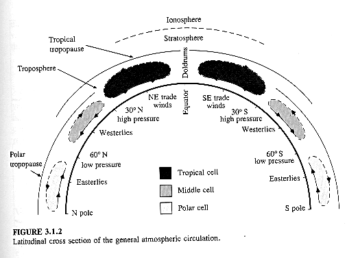
However, the earth does rotate, and the combined effects of the rotation of the earth and the poleward transport of heat energy are the driving forces behind the general circulation of the atmosphere which is shown in Chow, Maidment, and Mays, 1988, Figure 3.1.2.
The actual pattern of the atmospheric circulation has 3 cells: a tropical cell, a polar cell, and a middle cell, as well as jet streams and prevailing surface wind directions (See Dingman, 1994, Figure 3-8).
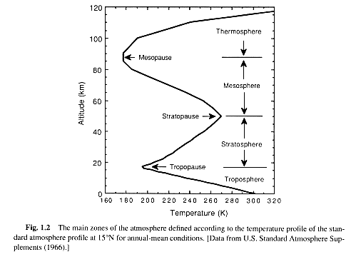
Hartmann (1994), Figure 1.2, shows that the atmosphere is divided vertically into various zones. The circulation described above occurs in the troposphere, which ranges in height from 8 km at the poles to 16 km at the equator. The troposphere accounts for more than 80% of the mass and virtually all of the water vapor, clouds, and precipitation in the earth's atmosphere. It is characterized by strong vertical mixing, e.g. in clear air it is not unusual for a parcel, or small control volume of air (containing water vapor) to travel the height of the troposphere in a few days (or minutes during a thunder storm).
In the troposphere, temperature decreases with altitude at a rate varying with its moisture content. The rate of decrease of tempereature with altitude in dry air is called the dry adiabatic lapse rate, and is roughly 9.8 deg C/km. Adiabatic implies no heat exchanged with surroundings. In moist air, the moist adiabatic lapse rate is typically half of the dry rate, or 5 deg C/km -- since the atmosphere is heated somewhat by the formation of precipitation. The average lapse rate in the troposphere is a weighted average of the dry and moist rates, and is roughly 6.5 deg C/km.
The top of the troposphere is called the tropopause. It is overlain by the stratosphere, stratopause, mesosphere, mesopause, etc.
3. Quantification of the amount of water vapor in the atmosphere
The atmosphere is a mixture of gases, each exerting a partial pressure proportional to its concentration, owing to its molecular motion and collision with other gases.
- The sum of the partial pressures of all the gases in the atmosphere is equal to the total atmospheric pressure.
- The partial pressure of water vapor is called the vapor pressure, e
The vapor pressure is computed from the ideal gas law as
e = rvRvTa
where
rv is the water vapor density (absolute humidity), i.e. the the mass concentration of water vapor in a volume of air;
Rv is the gas constant for water vapor; and
Ta is the air temperature
It can also be written in terms of atmospheric pressure, P, and the specific humidity, qv, (the mass of water vapor per unit mass of moist air rv/ra) as
e = qvP/.622
The maximum vapor pressure that is thermdynamically stable is called the saturation vapor pressure. It is a function of temperature only ( Dingman, 1994, Figure D-3) and can be computed as
esat(T) = 6.11 exp ((17.3 T)/(T+237.3))
where esat(T) is in mb and T in deg C.
A parcel of air at T and e below the esat(T) curve is unsaturated. The relative humidity, Wa of this parcel is the ratio of its actual vapor pressure to its saturation vapor pressure
Wa = e/esat
If the parcel is now cooled, as in Dingman (1994) Figure D-3, its saturation vapor pressure drops, so that its relative humidity increases. When the parcel is cooled to the point on the esat(T) curve it has reached its saturation vapor pressure, and its relative humidity of 100%.
The temperature to which a parcel with a given vapor pressure must be cooled in order to reach saturation is called the dew point
References
Dingman, S. L., 1994. Physical Hydrology, MacMillan Publishing Company, New York.
Hartmann, D. L. 1994. Global Physical Climatology, Academic Press, New York.
Back to top of page
5: Precipitation I
Outline
Precipitation is defined as the condensation of water to liquid or solid form, and subsequent falling to earth. It includes:
- rainfall
- snowfall
- hail
- sleet
- etc., i.e. any other processes by which water falls to earth
1. Requirements for formation of precipitation
In order for hydrologically significant rates of precipitation to occur, a sequence of several conditions must be met. These include
Air mass cooling
The formation of precipitation requires that an air mass be cooled to its dew point and some of its moisture condenses
An air mass in the general circulation is a large body of air that is fairly uniform horizontally in properties such as temperature and moisture content. Air masses are sub-continental in scale
- when an air mass moves slowly over land or sea, its characteristics reflect those of the underlying surface
- the region where an air mass acquires its characteristics is called its source region (e.g. tropics, poles)
Air masses can be cooled in a number of ways:
Cooling by these first four may result in fog or drizzle. Only vertical lifting can cause cooling high enough to produce significant amounts of rainfall.
From the ideal gas law we know that
P = rRT
and that pressure decreases with height into the atmosphere.
Therefore,
This is shown schematically in Dingman (1994) Figure D-6.
Condensation or freezing nuclei must be present
Condensation requires a seed called a condensation nucleus (cloud condensation nucleus or CCN) e.g. dust, particles containing ions like sea salt, sulfur and nitrogen from combustion) around which water molecules can attach themselves.
CCN are typically dust or particles containing ions. Major natural sources include
Natural concentrations of CCN are
Human activities can raise this number over land by a factor of 10 (e.g. combustion products including sulfur and nitrogen products that lead to acid rain)
Droplet formation and growth
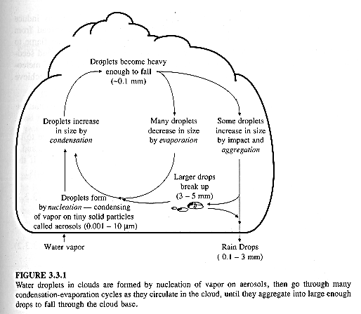
After condensing on CCN, drop size initially increases by continued condensation. Cloud droplets have sizes that range from 0.001 to 0.2 mm, and have fall velocities between 0.01 and 70 cm/s. For precipitation to fall from clouds, droplets must continue to grow to a size such that they are large enough so their terminal velocity is greater than the velocity of the updrafts that lifted them to the LCL, keeping in mind that there is evaporation as the drops start to fall. Therefore, the droplets must grow a few orders of magnitude to sizes on the order of 0.4 to 4 mm in diameter, or to snowflakes or even larger sizes.
Continued growth occurs by
• collision
• ice crystal growth
Collision: at temperatures above 0 deg C, produce droplets of varying sizes.
See Chow, Maidment, Mays (1988) Figure 3.3.1.
Ice crystal growth. In saturated air less than -40 deg C, vibrational energy of H20 molecules is low enough so that clusters of the molecules can spontaneously form ice crystals. When saturated air is between -40 and 0, a CCN with a molecular structure similar to that of ice is required to nucleate ice crystal growth. Given that some nucleation has occurred, since the saturation vapor pressure of ice is always lower than that of water for a given temperature below zero, water will evaporate from the liquid water and condense on the ice crystals. Growth continues in this fashion until the ice crystals are large enough to fall from the cloud.
Importation of Water Vapor
The concentration of liquid water and/or ice in most clouds is 0.1 to 1 g / m3. Consider a 10,000 m thick cloud, so that the total cloud volume over a m2 of ground is 10,000 m3.
If the concentration of water in the cloud is 0.5 g/m3 , the total volume of cloud water above each m2 is 5000 cm3. If all this water fell as precipitation, its depth would be 0.5cm, which is not much rain. Since most rain-producing clouds are less than 10,000 m in thickness, and water concentrations are less than 0.5 g/m3, a final requirement for the occurrence of significant amounts of precipitation is that a continual water vapor supply be imported to clouds to replace the rain that falls. This inflow of moisture is produced by winds that converge on precipitation producing clouds.
2. Mechanisms of air mass lifting
The three major mechanisms of air mass lifting include uplift due to
1. convergence
2. convection
3. orography
Convergence:
Airflow is induced by pressure gradients and movement is generally towards regions of low pressure. Looking back at the Dingman's Figure 3-8 we can imagine that high pressure regions are located where air descends from atmospheric cells, and low pressures where air is heated and rises. Thus low pressure areas are regions of convergence
• air converging from several directions is forced to rise
• adiabatic cooling results
• frontal convergence is characteristic of mid latitudes
• non-frontal convergence is a tropical phenomenon
Frontal convergence:. Outside of the tropics, in the mid latitudes, much of the precipitation results from frontal convergence (cyclonic convergence)
A cyclone is the convergence of air masses around a low pressure system.
• Air masses with contrasting temperatures, moisture contents and densities converge around the low
• The boundaries between air masses are called fronts
• In the northern hemisphere, the circulation is counterclockwise
• The diameter of a fully developed extratropical cyclone is about 1500 km
• Because of the temperature differences between the air masses, they tend not to mix, rather warm air is lifted over cold
Cold front: a cold air mass moves into a warm one characterized by
Warm front: a warm air mass displaces a cold one characterized by
Nonfrontal convergence. Convergence at the ITCZ: the low latitude Hadley cells create a tendency for convergence that circles the globe in tropical regions. This leads to adiabatic lifting and a band of heavy rain that circles the equator.
Tropical cyclones (Hurricanes) Tropical cyclones are non-frontal features and can develop into severe storms (hurricanes, typhoons, cyclonesm etc)
Uplift due to convection:
Convective precipitation results from adiabatic cooling when parcels of air at the surface are heated and rise because they are less dense. Look at Dingman (1994) Figure 4-7
Uplift due to orography
In most parts of the world, long-term mean precipitation increases with elevation (orographic effect)
Critical temperature for rain/snow transition.
Much of the precip that falls outside the tropics originates as snow or hail in supercooled clouds. The formation of precipitation reaching the surface is determined largely by the height of the 0 deg C surface. Rain occurs if the 0 deg surface is high enough so that the precipitation can melt before it reaches the ground
3. Moisture sources and transport
In the first half of the century, it was widely believed that most of the moisture falling as precipitation on a given land area entered the atmosphere as evaporation from the same or nearby areas.
However, starting around 1940, studies began to show that
More generally, precipitation over land is derived from two sources:
Recycled precipitation is defined as water that evaporates from land within a specified control volume and falls again as precipitation within the same control volume. We'll consider the remainder of the precipitation falling inside the control volume to be of advective origin (regardless of whether it was recently evaporated from an ocean or from the land surface outside the control volume).
Why is knowledge of vapor transport and recycling important?
For recent estimates of continental-scale precipitation recycling, see the papers by Brubaker et al (1993) including figures 1-6; and the review paper by Eltahir and Bras (1996).
References
Brubaker, K. L., D. Entekhabi and P. S. Eagleson, 1993. Estimation of Continental Precipitation Recycling, J. Clim., 1077-1089.
Dingman, S. L., 1994. Physical Hydrology, MacMillan Publishing Company, New York.
Eltahir, E. A. B. and R. L. Bras, 1996. Precipitation Recycling, Rev. Geophys., 367-368.
Back to top of page
6: Precipitation II
Outline
As an input to the land phase of the hydrological cycle, it is critical that we quantify the space-time variability of the precipitation falling to the earth's surface. Whether these problems are of local, small watershed, regional, continental, or global scale, we need to understand the amount of rainfall falling to the ground, and how that amount varies in space and time.
This problem has 2 components:
Types of precipitation gages
The principal behind measuring (gaging) precipitation is conceptually simple:
Recording rain gages
- automatically record rainfall accumulation down to 1 minute or less
- often equipped with telemetry so that real-time information can be transmitted
- includes:
weighing type --
Water collected is funneled to a vessel on a scale and the weight is recorded.
float and siphon type
A float rises as water level rises in the gage; height of the float is recorded.
tipping-bucket type
Water in the gage is funnelled to a pair of vessels with a known small capacity. When one vessel fills, it tips and drains, (bringing the other vessel into position) and the time of the tipping is recorded.
Non-recording rain gages
- generally a cylindrical container with a calibrated measuring stick.
- read and emptied once a day
- may be more elaborate with funnels and collecting vessels
Factors affecting measurement accuracy
To what degree is the gauge catch an accurate representation of the actual amount of precipitation that fell?
A number of issues need to be addressed:
- How big should the gage be?
- What should its shape be?
- Should it be placed level or parallel to the ground?
- Should it be shielded to minimize wind effects?
- Should it be fenced off to minimize disturbance by wildlife?
- How can evaporation be minimized?
There are no universal standards, and in fact, standards vary between countries. Dingman summarizes a number of studies which provide guidance on these issues.
Orifice size and orientation
- greater than 30 mm
- orifice should be level
Orifice height and wind shielding
- gages which are above ground cause turbulence which tends to reduce the catch of smaller rain drops and snowflakes. This is the most common cause of measurement error
- error increases with wind speed
- can be reduced by addition of wind shields or aerodynamic design
- lack of shielding can lead to 10% deficiencies for rain, 30% for snow
Distance to obstructions
Few studies have been done, but some general guidelines exist:
- best location is in an open space within a fairly uniform enclosure of trees, shrubs, fences, or other objects so that wind effects are minimized
- nothing should be located within the 45° conincal space centered on the gage
- individual obstructions (trees, buildings, etc) may produce wind eddies that can reduce gage catch and should not be closer than 2-4 times its height above the gage
Splash and evaporation
If the surface of the water in the gage is too close to the gage opening, the impact of falling drops can cause collected water to spash out. Prevent by
- deep gages
- vertical or outward sloping gage walls
- collecting caught water to a covered vessel
- frequent emptying
Limiting evaporation
- collecting caught water to a covered vessel
- frequent emptying
- add a nonvolatile immiscible oil that will prevent evaporation by floating on the collected water
Instrument errors
Systematic (mechanical) errors are common with recording rain gages
- e.g. tipping buckets often underrecord during heavy rains
- weighing gages have decreased sensitivity as weight of catch increases
- temperature can effect gage response
- the potential for mechanical/electrical failure always exists.
- It is normal to install a nonrecording gage to ensure as a minimum the total precip can be estimated
- Instrument errors can be on the order of 1-5% of the total catch
Observer errors
Very common but difficult to quantify
Can identify by periodically comparing record from a number of gages in the same region and noting outliers
- was there a thunderstorm to explain it?
- were there high streamflows locally to support it?
If an error, can correct objectively (statisically or otherwise)
Errors due to differences in observation time
e.g. in non-recording gages, observations are often daily
- the time of the observation varies widely
- so, could have yesterdays rainfall in today's reading
Errors due to occult precipitation
Occult precipitation: precipitation induced by cloud contact with trees or other vegetation.
- Not captured by normally sited precip gauges
- Can account for significant amounts of annual precip in high elevation or certain other environments
Fog drip is the liquid form and it occurs when clouds move through forests
- Cloud droplets are deposited on the leaf surfaces
- water drips to the ground
Rime is formed when supercooled clouds encounter exposed objects, like trees, and provide nucleation sites for ice-crystal formation and the buidup of ice, which ultimately falls to the ground as a solid or liquid
Errors due to low-intensity rains
Rain may enter gage, but not enough to measure accurately
- U.S. observers measure rainfall in standard nor-recording gages to the nearest 0.01 inch
- observation of less than 0.005 in is called a trace.
- Traces are counted as zero in totaling rainfall, so that if many traces are recorded, reported totals could be significantly less than actual totals
2. Checking the consistency of point measurements
Changes in type, location, or environment of a gage are common
- Buildings may be constructed nearby
- location may be changed
- urbanization can have important effects
These changes can significantly affect the gage catch
The hydrologist must determine whether the precipitation record is affected by such artificial changes and correct for them so they do not influence analyses. The most common technique for detecting and correcting for inconsistent precipitation data is by a double mass curve analysis. A double mass curve is a plot, on arithmetic graph paper, of the successive cumulative annual precipitation collected at a gage where measurement conditions may have changed, versus the successive cumulative annual precipitation for the same period of years collected at several gages in the same region (or the average of them).
A change in the proportionality between the measurements at a suspect station and those in the region is reflected as a change in slope. Dingman, Figure 4-20 displays double mass curve examples. The second graph in this figure indicates some inconsistency.
How are corrections made? General guidelines: the break in slope is only significant if it persists for 5 or more years, and then only if it is clearly associated with a change in measurement and it is determined to be statistically significant. Under these conditions, the annual values of the earlier part of the curve should be adjusted to be consistent with the later portions of the curve. Simply multiply the data for the period before the slope change by a factor K, where
K = slope for the period after the change/slope for the period before the change
Slope breaks in double mass curves can occur due to climatic shifts, so that adjustments should only be made if there is reason to believe that the break is due to a change in measurement conditions
References
Dingman, S. L., 1994. Physical Hydrology, MacMillan Publishing Company, New York.
Back to top of page
7: Precipitation III
Outline
Estimates of areally averaged precipitation are required at scales from the hillslope up to global.
If the true areal average is P, where
P = 1/A
![]() p(x,y) dx dy
p(x,y) dx dy
and A is the area of the region and p is
the precipitation falling at the coordinates x and y, then what
we're after is ![]() , the
estimated value of P.
, the
estimated value of P.
Approaches to the estimation of
![]() include
include
Direct weighted averages
Compute![]()
![]() directly
as a weighted average of measured values,
directly
as a weighted average of measured values,
where
and
pg are the precipitation values measured at each gage
Estimating the weights, vg:
Arithmetic average: Weights are equal to 1/G so that
Thiessen polygon
Construction of polygons
Surface-Fitting methods
Identify a surface which represents the spatial variability in precipitation which can be depicted on a map
General features:
where
![]() i is the average
precipitation value in the ith subregion
i is the average
precipitation value in the ith subregion
and ai is the area between the two contours
Contours can be drawn by hand (the eyeball isohyetal method) or automatically using specialized software. The software estimates the surface of precipitation given the gage values, and draws the contours on that surface.
These algorithms follow the following procedure
where
![]() j is the estimated
precipitation at the jth point, pg is the gage precipitation at station g, and
wjg is the weight assigned to a station g for point j.
j is the estimated
precipitation at the jth point, pg is the gage precipitation at station g, and
wjg is the weight assigned to a station g for point j.
• The difference between the various surface fitting methods is the manner by which the wjg are computed.
• Once the
![]() j 's are
computed, another algorithm is used to compute the contours
j 's are
computed, another algorithm is used to compute the contours
Important points regarding surface fitting:
Hypsometric method : good in regions where orographic effect is important
See Dingman (1994) figure 4-27
- Select an interval DZ and divide elevation range into H increments of DZ
- Determine the fraction of total area, ah within each increment of elevation
- Use the orographic equation to get
(z)h where (z)h is taken at the midpoint of each elevation increment
- Compute
as
2. Precipitation gage networks
Recommended gage density: see Dingman Table 4-5
In the US
278 primary stations
- staffed 24 hours by paid technicians
- located mainly at airports
8000 cooperative stations
operated by unpaid volunteers
Precipitation at these stations is recorded on at least a daily basis. Of these, hourly totals are recorded at 241 first order stations and 2600 cooperative stations. Many of these stations have been in operation for more than 100 years.
By 1996, a network of more than 120 high-quality radars, the Next Generation Weather Radar system, (NEXRAD) will be deployed in the U.S. This network will provide near complete coverage in the continental US.
Most important advantage of using radar for precipitation measurement
The NEXRAD systems are termed WSR-88D for weather surveillance radar, D is for Doppler. The radar unit transmits electromagnetic radiation (waves) of 10cm wavelength, and receives the returned signal, which is measured as
backscattered power, P,
P= C L Z / r2
which is related to characteristics of the radar and characteristics of the precipitation target.
P is related to
Measure P, know C, L, r, solve for Z. Determine rainfall rate from the a power law model
R = aZb
where the parameters a and b are determined using paired samples of reflectivity (from samples with known drop size distribution) and rainfall rate.
References
Back to top of page
8: Snow and Snowmelt I
Outline
The objective of this chapter is to become familiar with the physical characteristics of seasonal snowcover and the processes affecting them. Volumetrically, seasonal snowcover forms only a small fraction of the world's fresh water. Hydrologically, though , its importance is immense. Furthermore, it seasonally affects large portions of the landscape in North America.
In high and midlatitudes, and where precipitation is slight, melt of seasonal snow cover is the most significant hydrologic event of the year. In these regions, runoff from shallow snowcover can provide more than 80% of the annual surface runoff, as well as augment soil water reserves and recharge groundwater supplies
Even at lower latitudes, particularly in alpine regions, snowmelt is a primary source of water. For example, in California, as much as 85% to 90% of annual streamflow comes from spring snowmelt.
2. Formation and Interception.
Physics of formation.
We've previously discussed ice crystal formation: Continued growth of ice crystals leads to formation of snow crystals. A snow crystal is a large particle, having a very complex shape, and of such a size that it is visible to the naked eye. Their size and shape may change as they fall owing to freezing and accretion of water droplets with which they collide. This results in rimed crystals and in the extreme, snow pellets.
A snowflake is an aggregation of snow crystals that may also grow in size during its fall owing to the adhesion of colliding snow crystals. Whether a snowflake formed in the atmosphere arrives at the earth's surface as snow or rain depends on the height of the zero degree line above the earth's surface.
Interception
Interception of snowfall by vegetation canopies plays a major role in the snow hydrology of forests, including, the energy balance at the ground surface, the amount of snowfall lost to evaporation and sublimation, and the distribution of snow within a forest and forest openings
Interception occurs in the following manner. Early in a storm snowflakes fall through branches and needles until small bridged form at narrow openings. Bridges increase the collection area, and snow is retained on the bridges by cohesion. At some point a tree reaches its maximum holding capacity, when snow retention from subsequent snowfall is roughly balanced by the loss of intercepted snow falling to ground.
Morphological vegetation factors affecting interception include branch strength and flexure,
needle configuration and orientation, mass and surface area of vegetation, tree age and density. Interception by coniferous forests is much greater than by deciduous, as deciduous lose their leaves. Meteorological factors like air temperature and wind speed are generally of less importance than morphological characteristics
Wind effects interception by disrupting bridges, vibrating vegetation and thus reducing interception, erosion of intercepted snow and by retention of snow particles in suspension.
The amount of snow stored in the canopy continuously changes in response to wind erosion, evaporation and sublimation and melting.
3. Material characteristics of snow
The physical properties of a snowpack most important to hydrologists are depth, density, and snow water equivalent, the equivalent depth of water of a snow cover.
Snow is a granular porous medium consisting of ice and pore spaces. When snow is cold (i.e. when its temp is below 0°C) the pore spaces contain only air. At the melting point, the pore spaces contain liquid water as well as air (a 3-phase system)
For a snowpack of height hs and area A
Snow volume
Vs = Vi + Vw+ Va = hsA
Porosity is the ratio of pore volume to total volume
F = (Vw+ Va)/Vs
The liquid water content Q
Q = Vw/Vs
Snow density is the mass per unit volume of snow
rs = (Mi + Mw)/Vs
=(1-F )ri+Qrw
The water equivalent, hm, of the snow pack is the the depth of water that would result from completely melting the snow in place
hm = Vm/A
and Vm is the volume of meltwater, and can be shown to be equal to
hm = rs/rw hs
snow water equivalent equals relative density times depth
More on the density. Average density for new snowfall often assumed to be 100 kg/m3
However, in actuality, it varies with environment, though it is difficult to measure. In general, density depends upon the configuration of the snowflakes (i.e. the amount of air contained within the lattice of the snow crystals). Densities in the range of 50 to 120 kg/m3 are common. Lower values are associated with dry, cold conditions ane higher values found in wet snows at warm temperatures. Density is also a function of wind speed at the deposition surface. Higher winds tend to break up snowflakes so that they pack into denser layers. Maidment (1993), Fig 7.2.2 shows that thedensity of new fallen snow decreases exponentially as air temp decreases below freezing,
References
Dingman, S. L., 1994. Physical Hydrology, MacMillan Publishing Company, New York.
Maidment, D. R., 1993. Handbook of Hydrology, McGraw-Hill Publishing Co., New York.
Back to top of page
9: Infiltration and Redistribution I
Outline
1. Introduction to infiltration and terminology
In this chapter we'll discuss the movement of water through the unsaturated zone. Some of the processes we'll discuss are shown in Dingman (1994) Figure 6.1. Infiltration is the movement of water from the soil surface into the soil. Redistribution is the subsequent movement of infiltrated water in the unsaturated zone, vertically, laterally, etc. Percolation is the general term for downward flow in the unsaturated zone.
Redistribtution can also occur in an upward direction:
• exfiltration (evaporation)
• capillary rise (upward movement from the water table to the unsat zone under capillary, or surface tension forces)
• Plant uptake by roots
Lateral redistribution is called interflow
Importance of infiltration and redistribution of soil water: globally, 3/4 of the precipitation falling on land infiltrates so it is of great importance to the global cycle, e.g.
• via recharging soil moisture and ground water reservoirs
• soil water stored near the land surface is available to interact with the atmosphere and climate system.
• Provides all the water for natural and agriculture
We also need to understand infiltration and redistribution for water resource management purposes, including irrigation strategies, understanding the geochemistry of soils, forecasting runoff and flooding.
Let's begin our discussion of infiltration and redistribution by reviewing some of the material and hydraulic properties of soils
2. Material properties of soils
Distribution of pore and particle sizes
For the purposes of this class we'll consisder soil to be a matrix of solid grains (mineral or organic) between which are interconected pore spaces. Pores contain water and air in varying proportions
i.e. soil is a 3-phase system of solid mineral grains, water and air.
Pore size, or the size of pores through which water flows, is roughly equal to the grain size. The distribution of pore sizes is determined largely by the grain size.
Most soils have a mixture of grain sizes. Grain size distribution is often portrayed as a cumulative frequency plot of grain diameter vs weight fraction of grains with smaller diameter (See Dingman (1994) Figure 6-2).
Particle size distribution is further characterized by soil texture.
Texture is determined by the weight fraction of clay, sand, and silt
as shown in Dingman (1994) Figure 6-3. This is the USDA classification scheme for soil texture. Note that texture is determined by the fraction of silt, sand,clay after sand and larger particles have been removed. The weight fractions of soils of various diamters are meaured by sieve analysis.
Particle density is the mass of the mineral particles divided by the volume of the mineral particles
rm = Mm/Vm
Usually rm is not measured but estimated based on the composition of the soil. A value of 2.65 g/cm3 (the density of mineral quartz) is assumed for most soils.
Bulk density is the dry density of the soil
rb = Mm/Vs= Mm/(Va+Vw+Vm)
Bulk density increases with depth owing to compaction by weight of overlying soil.
Porosity, f, is the ratio of the volume of voids to the total volume
f = (Va+Vw)/Vs
Porosity decreases with depth owing to compaction, and owing to the presence of macropores near the surface.
Dingman (1994) Figure 6-4 shows a range of porosity values for different soil textures, and Figure 6-5 provides the basis ofr explanation in terms of the packing arrangement of clay particles vs. sand particles for range of porosities and explanation
Volumetric water content
q = Vw/Vs
Measurement in the lab consists of weighing a sample of known volume, oven drying it at 105 deg C, and re-weighing, then calculating
q = (Mswet - Msdry)/rwVs
where Ms stands for mass of soil
Degree of saturation (relative saturation) is the volume of water normalized by the porosity
S = Vw / (Va + Vw) = q / f
References
Back to top of page
10: Infiltration and Redistribution II
Outline
1. Other soil moisture measurement techniques
2. Hydraulic Properties of Soils
Flows in unsaturated porous media are described by Darcy's Law
Vx = -Kh d(z+ p/gw)/dx
where
so that
Vx = -Kh dh/dx
In unsaturated flows, both the pressure head and the hydraulic conductivities are functions of the soil water content, Q, so that
Vx = -Kh(q) d(z + y(q))/dx
Let's look at K-q and y-q relations in the unsaturated zone in a little more detail. The simplest hydrologic configuration of saturated and unsaturated conditions is that of an unsaturated zone overlying a capillary fringe and a saturated zone. The water table is defined as the surface on which the fluid pressures p in the pores of a porous medium is exactly atmospheric. If p is measured in gage pressure, then on the water table, p = 0 which implies that y = 0. From your groundwater classes, in the saturated zone we know that both y and p are > 0. In the unsaturated zone, both y and p are < 0 which reflects the fact that water in the unsaturated zone is held in the soil pores under surface tension forces
A microscopic inspection would reveal a concave meniscus extending from grain to grain across each pore channel. The radius of curvature on each mensicus reflects the surface tension on that individual, microscopic, air-water interface. In reference to the physical mechanism of water retention, soil physicists often call the negative pressure the tension head, or head
Again, from your groundwater class, you've probably discussed that piezometers are used to measure head in the saturated zone. However,above the water table, where y < 0 , we use tensiometers to measure y in the unsaturated zone.
A tensiometer consists of a porous cup attached to an airtight, water-filled tube. The porous cup is inserted into the soil at the desired depth, and allowed to reach a hydraulic equilibrium. The equilibration involves the passage if water through the porous cup from the tube into the soil. The vacuum created at the top of the airtight tube is a measure of the pressure head in the soil. It is usually measured by a vacuum gage attached to the tube above the ground surface. To obtain total head, h, the negative y is added to the elevation head z at the point of measurement.
3. Pressure-Water Content relations
Pressure head
The relationship between pressure head, y, and moisture content, q,
for a given soil is called the moisture characteristic curve. The relationship is highly nonlinear, and typically of the form shown in Dingman, Figure 6-7. Note that pressure head is zero when water content equals the porosity.
Water content changes little as tension increases up to a point of inflection. This rather distinct point represents the tension at which significant volumes of air begin to appear in soil pores, and is called the air entry tension, or air entry suction head, yae. The absolute value of the air-entry suction head equals the height of the capillary fringe, or the height of the tension saturated zone. As tension increases to very high levels, the curve becomes nearly vertical reflecting a residual water content that is very tightly held in soil pores by capillary forces.
In real soils, the value of tension at a given water content is not unique and depends on the soil's wetting a drying history. Hysteresis can have a significant influence on soil moisture movement but it is difficult to model mathematically, and is often left out of hydrological models. See Figure 6-9 from Dingman (1994)
Hydraulic Conductivity
Hydraulic conductivity is the rate at which water moves through a porous medium under a unit hydraulic gradient. Under saturated conditions
K = krg/m
Under unsaturated conditions K is also a function of the degree of saturation of the soil -- the wetter the soil, the more interconnected flow paths. See figure 6-7 of Dingman (1994).
The relationships between y-q and K-q can be expressed parametrically
|y(S)| = |ys|S-b
Kh(S) =KhsatSc
where
Values of these parameters are functions of soil texture and are tabulated as averages over many soils in the literature.
Summary of saturated, unsaturated and tension saturated zones
Saturated
Unsaturated
Capillary fringe
4. Water Conditions in Natural Soils
Soil water status
If a soil is saturated, then allowed to drain without being subject to evaporation, plant uptake and capillary rise, its water content will decrease exponentially. Within a few days, the soil will reach a value beyond which a further decrease in moisture content (drainage) occurs very slowly. This value is known as the field capacity qfc. It represents the water that can be held against gravity. The pressure head at field capacity is close to - 340 cm for most soils.
After a soil has reached field capacity, water can only be removed by direct evaporation or by plant uptake. However, plants can't exert suctions stronger than -15,000 cm. When water content is reduced to this point on the moisture characteristic curve, transpiration ceases and plants wilt. This point is known as the permanent wilting point qpwp. It ranges from 0.05 for sands to 0.25 for clays.
The difference between the field capacity and pwp is the water available for plant use (available water content, qa)
These concepts are shown schematically in Dingman (1994) Figure 6-12.
References
Back to top of page
11: Infiltration and Redistribution III
Outline
1. Pressure-Water Content Relations
Pressure head
The relationship between pressure head, y, and moisture content, q,
for a given soil is called the moisture characteristic curve. The relationship is highly nonlinear, and typically of the form shown in Dingman, Figure 6-7. Note that pressure head is zero when water content equals the porosity.
Water content changes little as tension increases up to a point of inflection. This rather distinct point represents the tension at which significant volumes of air begin to appear in soil pores, and is called the air entry tension, or air entry suction head, yae. The absolute value of the air-entry suction head equals the height of the capillary fringe, or the height of the tension saturated zone. As tension increases to very high levels, the curve becomes nearly vertical reflecting a residual water content that is very tightly held in soil pores by capillary forces.
In real soils, the value of tension at a given water content is not unique and depends on the soil's wetting a drying history. Hysteresis can have a significant influence on soil moisture movement but it is difficult to model mathematically, and is often left out of hydrological models. See Figure 6-9 from Dingman (1994)
Hydraulic Conductivity
Hydraulic conductivity is the rate at which water moves through a porous medium under a unit hydrualic gradient. Under saturated conditions
K = krg/µ
Under unsaturated conditions K is also a function of the degree of saturation of the soil -- the wetter the soil, the more interconnected flow paths. See figure 6-7 of Dingman (1994). Freeze and Cherry (1979) Figure 2-14 shows effects of different soil textures
The relationships between y-q and K-q can be expressed parametrically
|y(S)| = |ys|S-b
Kh(S) =KhsatSc
where
Values of these parameters are functions of soil texture and are tabulated as averages over many soils in the literature.
Summary of saturated, unsaturated and tension saturated zones
Saturated
Unsaturated
2. Water Conditions in Natural Soils
Soil water status
If a soil is saturated, then allowed to drain without being subject to evaporation, plant uptake and capillary rise, its water content will decrease exponentially. Within a few days, the soil will reach a value beyond which a further decrease in moisture content (drainage) occurs very slowly. This value is known as the field capacity qfc. It represents the water that can be held against gravity. The pressure head at field capacity is close to - 340 cm for most soils.
After a soil has reached field capacity, water can only be removed by direct evaporation or by plant uptake. However, plants can't exert suctions stronger than -15,000 cm. When water content is reduced to this point on the moisture characteristic curve, transpiration ceases and plants wilt. This point is known as the permanent wilting point qpwp . It ranges from 0.05 for sands to 0.25 for clays.
The difference between the field capacity and pwp is the water available for plant use (available water content, qa)
These concepts are shown schematically in Dingman (1994) Figure 6-12, and in a vertical soil column in Figure 6-13.
References
Back to top of page
12: Infiltration and Redistribution IV
Outline
1. Qualitative description at a point
Infiltration is the process by which water arriving at the soil surface enters the soil. Let's review some terminology found in the text and look at things qualitatively before moving on to quantitative description.
Dingman (1994) defines the beginning of a water-input event begins a t time t = 0 and ending at t = tw. The infiltration rate f(t), or(actual infiltration rate) is the rate at which water enters the soil from the surface. The water input rate w(t) is the rate at which water arrives at the surface due to rain or snowmelt. The infiltration capacity fc(t) is the maximum rate at which infiltration can occur. The depth of ponding Y(t), the depth of water standing on the surface.
Then 3 conditions are recognized which control the actual infiltration rate:
1.) No ponding. The water input rate is less than the infiltration capacity, so that all water infiltrates and none ponds on the surface. The actual infiltration rate is equal to the water input rate.
Y(t) = 0 f(t) = w(t)
2.) Saturation fom above. Ponding has occurred because the water input rate is greater thatn the infiltration capacity. The actual infiltration rate proceeds at the infiltration capacity.
Y(t) > 0 f(t) = fc(t)
3.) Saturation from below. The water table has risen to or above the surface and the entire soil is saturated. Soil pores are full and there is no room for infiltrated water.
Y(t)
![]() 0 f(t) = fc(t)
= 0
0 f(t) = fc(t)
= 0
Based the above we can state that the actual infiltration rate is equal to the minimum of the water input rate or the infiltration capacity.
f(t) = min [ w(t), fc(t)]
Ring infiltrometer.
The ring infiltrometer is a cylindrical ring,which is driven into the ground, flooded, and the level of water in the ring ismonitored to determine the infiltration rate.
The ring is first flooded, then the infiltration rate is obtained by measuring the rate at which the level of ponded water decreases, or by measuring the rate at which water must be added to maintain constant head.
In general, during a water input event, infiltration rates start out high and decrease exponentially with time into a storm, ultimately approaching a constant rate which is equal to Ksat.
Because infiltrating water encounters both capillary and gravitational forces, the water beneath the ring moves laterally as well as vertically, so that the measured infiltration rate often exceeds the rate if the entire surface were ponded. A double-ring infiltrometer can be used to set up a buffer zone and obtain a more realistic estimate of infiltration. Alternatively, a capillary correction term can be applied.
Sprinkler plot
A sprinkler is applied to a plot of land surface at a known rate. Runoff is measured. The difference between the water applied and the runoff is infiltrated water.
Observation of soil water
Install a nest of tensiometers which monitor pressure head at different levels. Pressures can be converted to moisture content using the moisture characteristic equations (remembering problems with hysteresis) and the depth and rate of infiltration can be determined from analysis of the profiles.
References
Back to top of page
13: Infiltration and Redistribution V
Outline
1. Basic characterisitics of infiltration
In general, the infiltration capacity decreases with time into an event, and ultimately approaches the saturated hydraulic conductivity. At early times into an event, capillary forces dominate infiltration. However, these forces decrease with time as the soil wets, until eventually, gravitational forces dominate.
Figure xx shows another characteristic of an infiltration event, the formation of a wetting front near the soil surface...
2. Factors affecting infiltration rate
f(t) is determined by affects of gravity and pressure forces arriving at the surface, which in turn are determined by the
- 1. Rate of arrival of water at the surface, or depth of ponding
- 2. Khsat at the surface
- 3. Initial soil wetness
- 4. Inclination and surface roughness
- 5. Chemical characteristics of the soil surface
- 6. Physical and chemical properties of water
The first of these has already been discussed.
Khsat at the surface
organic surface layers: Litter, humus and other organic material where has a loose, open structure with a high hydraulic conductivity regardless of texture of the underlying mineral soil. Root growth, insects and burrowing mammals contribute to the surface porosity.
frost: High water content at the surface can render soil impermeable upon freezing. Frost associated with lower water contents can increase conductivity by producing crack networks, e.g. polygonal cracks.
swelling and drying: Clay minerals can swell and shrink during rain events. Swelling can reduce permeabiliy, porosity, and limit infiltration during dry periods. Crack networks can develop that can result in high infiltration rates.
inwashing of fine sediments: Fine sediments may wash into soil pores reducing effective pore size and permeability.
human impact. Depends on the nature of the activity. Plowing may increase but grazing, other heavy equipment may compact soil.
Initial soil wetness
As mentioned previously, saturation from below eliminates infiltration. This occurs under rising water table conditions, or also from decreased hydraulic conductivity at depth which encourages a build-up of water from below.
In unsaturated soils, high water contents tend to increase Khsat and thus infiltration rates. However, higher water contents reduce the effects of surface tension/capillary forces.
The net effect of antecedent water thus depends on the water input rate and duration, the distribution of soil hydraulic conductivity with depth, depth of the local water table and initial water contnent
Surface slope and roughness
Steeper, smoother slopes limit depth of ponding and thus infiltration rates.
Chemical characteristics of the soil surface Some vegetation produces waxy organic substances which renders soils hydrophobic, i.e. water beads up, and thus infiltration is limited. This is a minor effect under undisturbed conditions, but more significant when, e.g. organic layers are burned off in forest fires and the waxy substances condenses on bare soil.
Physical/chemical properties of water For example, viscosity is very temperature sensitive: higher viscosity occur at lower temperatures, and thus infiltration rates are lower.
3. Spatial variability of infiltration
Infilitration at a point is controlled by: soil type and properties (porosity, Khsat, air entry suction head, pore size distribution), initial moisture content and rainfall rates. As we move from the point to the hillslope to the catchment and greater scales, we encounter spatial variability in soils, moisture content and rainfall patterns, and consequently spatial variability in infiltration rates. The degree of the variability is simply a function of the amount of variability of the individual patterns listed above and how they interact. The book describes various attempts at modeling but in fact, at the catchment scale, the most direct approach is spatially-distributed modeling. At larger scales, statistical methods may be more appropriate.
References
Back to top of page