![]()
Merge Sort
![]()
![]()
![]()
Merge sort is based on the divide-and-conquer paradigm. Its worst-case running time has a lower order of growth than insertion sort. Since we are dealing with subproblems, we state each subproblem as sorting a subarray A[p .. r]. Initially, p = 1 and r = n, but these values change as we recurse through subproblems.
To sort A[p .. r]:
1. Divide Step
If a given array A has zero or one element, simply return; it is already sorted. Otherwise, split A[p .. r] into two subarrays A[p .. q] and A[q + 1 .. r], each containing about half of the elements of A[p .. r]. That is, q is the halfway point of A[p .. r].
2. Conquer Step
Conquer by recursively sorting the two subarrays A[p .. q] and A[q + 1 .. r].
3. Combine Step
Combine the elements back in A[p .. r] by merging the two sorted subarrays A[p .. q] and A[q + 1 .. r] into a sorted sequence. To accomplish this step, we will define a procedure MERGE (A, p, q, r).
Note that the recursion bottoms out when the subarray has just one element, so that it is trivially sorted.
Algorithm: Merge Sort
To sort the entire sequence A[1 .. n], make the initial call to the procedure MERGE-SORT (A, 1, n).
MERGE-SORT (A, p, r)
1. IF p < r // Check for base case
2. THEN q = FLOOR[(p +
r)/2] // Divide step
3. MERGE (A,
p, q) // Conquer step.
4. MERGE (A,
q + 1, r) // Conquer step.
5. MERGE (A,
p, q, r) // Conquer step.
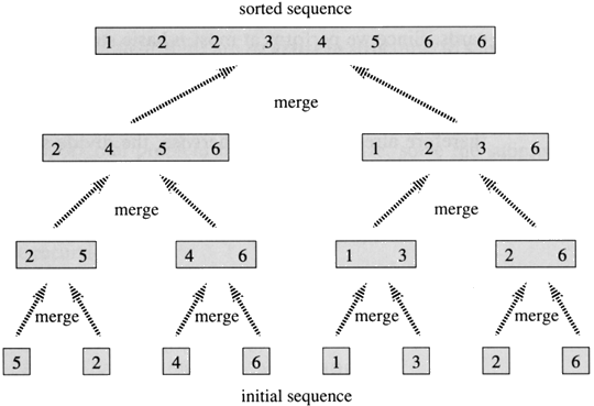
Example: Bottom-up view of the above procedure for n = 8.
Merging
What remains is the MERGE procedure. The following is the input and output of the MERGE procedure.
INPUT: Array A and indices p, q, r such that p ≤ q ≤ r and subarray A[p .. q] is sorted and subarray A[q + 1 .. r] is sorted. By restrictions on p, q, r, neither subarray is empty.
OUTPUT: The two subarrays are merged into a single sorted subarray in A[p .. r].
We implement it so that it takes Θ(n) time, where n = r − p + 1, which is the number of elements being merged.
Idea Behind Linear Time Merging
Think of two piles of cards, Each pile is sorted and placed face-up on a table with the smallest cards on top. We will merge these into a single sorted pile, face-down on the table.
A basic step:
Choose the smaller of the two top cards.
Remove it from its pile, thereby exposing a new top card.
Place the chosen card face-down onto the output pile.
Repeatedly perform basic steps until one input pile is empty.
Once one input pile empties, just take the remaining input pile and place it face-down onto the output pile.
Each basic step should take constant time, since we check just the two top cards. There are at most n basic steps, since each basic step removes one card from the input piles, and we started with n cards in the input piles. Therefore, this procedure should take Θ(n) time.
Now the question is do we actually need to check whether a
pile is empty before each basic step?
The answer is no, we do not. Put on the bottom of each input pile a special
sentinel card. It contains
a special value that we use to simplify the code. We use ∞, since that's
guaranteed to lose to any other value. The only way that ∞ cannot lose is when
both piles have ∞ exposed as their
top cards. But when that happens, all the nonsentinel cards have already been
placed into the output pile.
We know in advance that there are exactly r − p + 1 nonsentinel cards so stop
once we have performed r − p + 1 basic steps. Never a need to check for
sentinels, since they will always lose. Rather than even counting basic steps,
just fill up the output array from index p
up through and including index r .
The pseudocode of
the MERGE procedure is as follow:
MERGE (A, p, q, r )
1. n1 ← q − p + 1
2. n2 ← r − q
3. Create arrays L[1 . . n1 + 1] and R[1 . .
n2 + 1]
4. FOR i ← 1 TO
n1
5. DO L[i] ← A[p +
i − 1]
6. FOR j ← 1 TO
n2
7. DO R[j] ← A[q +
j ]
8.
L[n1 + 1] ← ∞
9.
R[n2 + 1] ← ∞
10. i ← 1
11. j ← 1
12. FOR k ← p TO
r
13. DO IF L[i
] ≤ R[
j]
14.
THEN A[k] ← L[i]
15.
i ← i + 1
16.
ELSE A[k] ← R[j]
17.
j ← j + 1
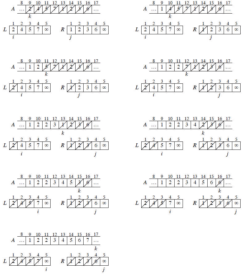
Example [from CLRS-Figure 2.3]: A call of MERGE(A, 9, 12, 16). Read the following figure row by row. That is how we have done in the class.
The first part shows the arrays at the start
of the "for k ← p to r" loop, where
A[p . . q] is copied into L[1 . . n1]
and A[q + 1 . . r ] is
copied into R[1 . . n2].
Succeeding parts show the situation at the start of successive iterations.
Entries in A with slashes have had their values copied to either L or R and have not had a value copied back in yet. Entries in L and R with slashes have been copied back into A.
The last part shows that the subarrays are merged back into A[p . . r], which is now sorted, and that only the sentinels (∞) are exposed in the arrays L and R.]
Running Time
The first two for loops (that is, the loop in line 4 and the loop in line 6) take Θ(n1 + n2) = Θ(n) time. The last for loop (that is, the loop in line 12) makes n iterations, each taking constant time, for Θ(n) time. Therefore, the total running time is Θ(n).
Analyzing Merge Sort
For simplicity, assume that n is a power of 2 so that each divide step yields two subproblems, both of size exactly n/2.
The base case occurs when n = 1.
When n ≥ 2, time for merge sort steps:
Divide: Just compute q as the average of p and r, which takes constant time i.e. Θ(1).
Conquer: Recursively solve 2 subproblems, each of size n/2, which is 2T(n/2).
Combine: MERGE on an n-element subarray takes Θ(n) time.
Summed together they give a function that is linear in n, which is Θ(n). Therefore, the recurrence for merge sort running time is

Solving the Merge Sort Recurrence
By the master theorem in CLRS-Chapter 4 (page 73), we can show that this recurrence has the solution
T(n) = Θ(n lg n).
Reminder: lg n stands for log2 n.
Compared to insertion sort [Θ(n2) worst-case time], merge sort is faster. Trading a factor of n for a factor of lg n is a good deal. On small inputs, insertion sort may be faster. But for large enough inputs, merge sort will always be faster, because its running time grows more slowly than insertion sorts.
Recursion Tree
We can understand how to solve the merge-sort recurrence without the master theorem. There is a drawing of recursion tree on page 35 in CLRS, which shows successive expansions of the recurrence.
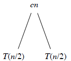
The following figure (Figure 2.5b in CLRS) shows that for the original problem, we have a cost of cn, plus the two subproblems, each costing T (n/2).
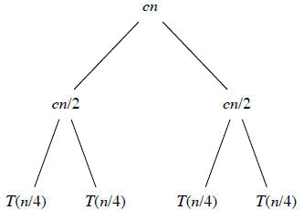
The following figure (Figure 2.5c in CLRS) shows that for each of the size-n/2 subproblems, we have a cost of cn/2, plus two subproblems, each costing T (n/4).
The following figure (Figure: 2.5d in CLRS) tells to continue expanding until the problem sizes get down to 1.
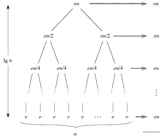
In the above recursion tree, each level has cost cn.
The top level has cost cn.
The next level down has 2 subproblems, each contributing cost cn/2.
The next level has 4 subproblems, each contributing cost cn/4.
Each time we go down one level, the number of subproblems doubles but the cost per subproblem halves. Therefore, cost per level stays the same.
The height of this recursion tree is lg n and there are lg n + 1 levels.
Mathematical Induction
We use induction on the size of a given subproblem n.
Base case: n = 1
Implies that there is 1 level, and lg 1 + 1 = 0 + 1 = 1.
Inductive Step
Our inductive hypothesis is that a tree for a problem size of 2i has lg 2i + 1 = i +1 levels. Because we assume that the problem size is a power of 2, the next problem size up after 2i is 2i + 1. A tree for a problem size of 2i + 1 has one more level than the size-2i tree implying i + 2 levels. Since lg 2i + 1 = i + 2, we are done with the inductive argument.
Total cost is sum of costs at each level of the tree. Since we have lg n +1 levels, each costing cn, the total cost is
cn lg n + cn.
Ignore low-order term of cn and constant coefÞcient c, and we have,
Θ(n lg n)
which is the desired result.

Implementation
void mergeSort(int numbers[], int temp[], int array_size)
{
m_sort(numbers, temp, 0, array_size -
1);
}
void m_sort(int numbers[], int temp[], int left, int right)
{
int mid;
if (right > left)
{
mid = (right
+ left) / 2;
m_sort(numbers,
temp, left, mid);
m_sort(numbers,
temp, mid+1, right);
merge(numbers, temp, left, mid+1, right);
}
}
void merge(int numbers[], int temp[], int left, int mid, int right)
{
int i,
left_end, num_elements, tmp_pos;
left_end =
mid - 1;
tmp_pos =
left;
num_elements
= right - left + 1;
while ((left <= left_end) && (mid <= right))
{
if (numbers[left] <= numbers[mid])
{
temp[tmp_pos] = numbers[left];
tmp_pos = tmp_pos + 1;
left = left +1;
}
else
{
temp[tmp_pos] = numbers[mid];
tmp_pos = tmp_pos + 1;
mid = mid + 1;
}
}
while (left <=
left_end)
{
temp[tmp_pos] = numbers[left];
left = left + 1;
tmp_pos = tmp_pos + 1;
}
while (mid <= right)
{
temp[tmp_pos] = numbers[mid];
mid = mid + 1;
tmp_pos = tmp_pos + 1;
}
for (i = 0; i <= num_elements; i++)
{
numbers[right] = temp[right];
right = right - 1;
}
}
Update: January 14, 2010.